Flow / Begin with a vortex you can check
Recover velocity from one scalar field
One evolving vorticity field. A Poisson solve supplies its velocity.
Download runnable lesson (.zip)
Includes the model, inputs, required headers and a short run guide.
A two-dimensional incompressible flow can be described by the scalar vorticity \(\omega\). The retained OpenPFC prototype advances
\[ \omega_t+\mathbf u\cdot\nabla\omega=\nu\nabla^2\omega, \]
and recovers a streamfunction and velocity through
\[ \begin{aligned} \nabla^2\psi&=-\omega,\\ \mathbf u&=(\psi_y,-\psi_x). \end{aligned} \]
The velocity is divergence free because the two mixed derivatives cancel. On a periodic grid, Fourier differentiation and a diagonal Poisson solve make this relationship explicit; Trefethen (2000) supplies the spectral background. This chapter teaches the existing solver rather than introducing a second flow implementation.
Compose the field, transform and equation
pfc::sim::stacks::SpectralCPUStack stack(ns2d::make_slab(cli.n, length), rank,
                                         nproc, MPI_COMM_WORLD);
ns2d::VorticityStreamCPU solver(stack, ns2d::Params{cli.nu, dt});
SpectralCPUStack owns the field and distributed FFT plan. The example’s VorticityStreamCPU composes Poisson recovery, derivatives and the integrating-factor step. Its slab is \(N\times N\times1\), so \(k_z=0\); the physical example remains two dimensional.
For a nonzero mode,
\[ \widehat\psi_{\mathbf k}=\widehat\omega_{\mathbf k}/|\mathbf k|^2. \]
The streamfunction’s zero mode is set to zero, fixing an arbitrary additive constant. This does not set mean vorticity to zero. The solver retains that mode and gives the nonlinear tendency zero DC. All supplied periodic initial conditions have zero mean vorticity, as a curl of a periodic velocity must. Odd derivative symbols suppress the Nyquist component consistently.
Look inside the nonlinear evaluation
void nonlinear_from_hat(const std::vector<Complex> &omega_hat,
                        std::vector<Complex> &n_hat) {
  m_plane.poisson(omega_hat, m_psi_hat);
  m_plane.curl_from_hat(m_psi_hat, m_u, m_v);
  m_plane.invert_ik(omega_hat, m_plane.kx_odd(), +1.0, m_wx);
  m_plane.invert_ik(omega_hat, m_plane.ky_odd(), +1.0, m_wy);
  for (std::size_t i = 0; i < m_n.size(); ++i) {
    m_n[i] = -(m_u[i] * m_wx[i] + m_v[i] * m_wy[i]);
  }
  m_plane.fft().forward(m_n, n_hat);
  m_plane.project_hat(n_hat);
  m_plane.zero_dc(n_hat);
}
First recover velocity from vorticity. Then compute both vorticity derivatives and form \(-(u\omega_x+v\omega_y)\) at owned nodes. Transform that product back and project it onto the retained Fourier band.
The two-thirds mask applies to the state and every integrating-factor RK4 stage before products, as well as to the resulting tendency. Masking only the product would allow discarded input modes to alias into the retained band. This is a quadratic product, unlike the cubic projection lesson.
Start with a vanishing advection term
Use the periodic square \([0,2\pi)^2\) and the exact Taylor–Green field
\[ \omega(x,y,t)=2\sin x\sin y\,e^{-2\nu t}. \]
[[nodiscard]] inline double taylor_green_omega(double x, double y, double nu,
                                               double t) noexcept {
  return 2.0 * std::sin(x) * std::sin(y) * std::exp(-2.0 * nu * t);
}
Here \(\nabla^2\omega=-2\omega\), while \(\mathbf u\cdot\nabla\omega=0\): the two product terms cancel. The integrating factor therefore advances this mode exactly up to floating point error. With spatial averages over the square, kinetic energy and half the mean squared vorticity are
\[ \begin{aligned} E(t)&=\tfrac14 e^{-4\nu t},\\ Z(t)&=\tfrac12 e^{-4\nu t}. \end{aligned} \]
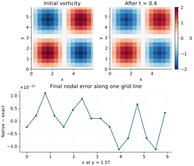
The plots read the C++ binary snapshots. Both maps use the same color scale, and the final curve compares actual nodal output with the exact mode. Output checks inspect every point in both snapshots, rather than just the displayed line. The CSV diagnostics use six significant digits; that printed precision is distinct from the binary field’s precision.
This checks normalization, derivative signs, Poisson recovery and viscous decay. It does not establish nonlinear fourth-order time accuracy, because this particular advection term vanishes. A two-mode case is needed for that separate question.
Compile the shared example and verify it
From the repository root, with a compatible installed spectral CPU SDK:
mkdir -p results
openpfc compile examples/flow/vorticity/model.cpp --source-root examples/flow -o results/vorticity
results/vorticity --verify --N 16 --steps 8 --dt 0.05 --nu 0.1 --outdir results/flow/vorticity
The source compiler captures quoted dependencies below the declared flow root. The model shares cases.hpp, vorticity_stream.hpp and spectral.hpp. Keep that relative layout when using downloaded files; the checkout already supplies it.
--verify compares the final field with the exact vortex using the retained \(10^{-9}\) maximum-error criterion. The run writes diagnostics, metadata and field snapshots beneath the selected result directory. The CMake executable name remains ns2d_vorticity, with its existing verification tests and build location.
Change --nu or the final time and predict the energy decay before running. Then try --case two_mode without --verify to activate nonlinear transfer. Keep that experiment separate from the exact-vortex check: a plausible flow picture alone does not establish correctness. The double-shear case uses a unit square, not this \(2\pi\) square; its length and viscosity conventions must be preserved when experimenting.