Solve a weak equation on free nodes

Finite elements / Integrate the load, then solve the discrete equation

Solve a weak equation on free nodes

A tensor-product basis. A matrix-free action. Two different errors to measure.

Download runnable lesson (.zip)

Includes the model, inputs, required headers and a short run guide.

On the unit cube, consider

\[ -D\nabla^2u+cu=f,\qquad u|_{\partial\Omega}=0, \]

with constant \(D>0\) and \(c\ge0\). Choose the continuum solution

\[ s(x,y,z)=\sin(\pi x)\sin(\pi y)\sin(\pi z), \]

so \(f=(3D\pi^2+c)s\). Finite elements approximate the weak equation: for each test function \(v\) vanishing on the boundary,

\[ D\int_\Omega\nabla u_h\cdot\nabla v +c\int_\Omega u_hv=\int_\Omega fv. \]

Here \(u_h\) uses continuous trilinear, or Q1, basis functions on a uniform hexahedral mesh. Brenner and Scott (2008) gives the finite-element background. The installed OpenPFC hierarchy supplies the Q1 action and multigrid cycle; the example does not implement a second assembler.

Store only the free coefficients

With \(n+1\) elements per axis and \(h=1/(n+1)\), the free nodes have coordinates \(h,2h,\ldots,nh\). The physical boundary coefficients are zero and eliminated. The field domain therefore contains \(n^3\) free coefficients, beginning at physical origin \((h,h,h)\):

const auto domain =
    pfc::domain::create(pfc::GridSize{{n, n, n}}, pfc::PhysicalOrigin{{h, h, h}},
                        pfc::GridSpacing{{h, h, h}}, {false, false, false});
const auto decomposition =
    pfc::decomposition::create(domain, pfc::Int3{comm.size(), 1, 1});
const auto box = pfc::decomposition::local_box(decomposition, comm.rank());
using Operations = pfc::solvers::FieldOperations<pfc::HostSpace>;
Operations operations(domain, box, 1, 1, comm);
auto rhs = operations.make(operations.size());
auto solution = operations.make(operations.size());

The declared axes are nonperiodic. FieldOperations supplies owned-node algebra and collective norms for a single field with one halo cell. The hierarchy owns the communication needed by its actions and transfers.

This bounded example uses \(n=15\) or \(31\), with one or two MPI ranks. Both have the supported form \(2^k-1\). They coarsen to seven free nodes per axis: \(15\to7\) or \(31\to15\to7\). Only the bounded \(7^3=343\)-unknown coarse solve is replicated; the fine operator acts on distributed owned nodes.

Integrate the forcing against the basis

The right-hand side is a basis integral, rather than a pointwise sample of \(f\). For the one-dimensional hat function \(\phi_i\),

\[ \int_0^1\sin(\pi x)\phi_i(x)\,dx =\beta\sin(\pi x_i), \]

where

\[ \beta=\frac{2(1-\cos(\pi h))}{h\pi^2}. \]

Tensor-product separation gives the three-dimensional load:

auto sine = [=](double x, double y, double z) {
  return std::sin(pi * x) * std::sin(pi * y) * std::sin(pi * z);
};
const double beta = 2 * (1 - std::cos(pi * h)) / (h * pi * pi);
const double load = (3 * diffusion * pi * pi + reaction) * beta * beta * beta;
rhs[0].apply([&](double x, double y, double z) { return load * sine(x, y, z); });

The factor \(\beta^3\) carries the integrated basis measure. Omitting it, or silently replacing it with a pointwise forcing, changes the discrete equation and its expected coefficients.

Compose the installed multigrid and CG interfaces

using Multigrid = pfc::solvers::NodalDirichletMultigrid;
Multigrid::Controls settings;
settings.diffusion = diffusion;
settings.reaction = reaction;
Multigrid hierarchy(decomposition, comm.rank(), comm, settings);
pfc::solvers::KrylovControls controls;
controls.relative_tolerance = 1e-12;
controls.maximum_iterations = 120;
const auto status = pfc::solvers::cg(
    operations,
    [&](const auto &x, auto &out) { hierarchy.apply_operator(x[0], out[0]); },
    rhs, solution, controls,
    [&](const auto &r, auto &out, int) { hierarchy.apply(r[0], out[0]); });
if (!status.converged())
  throw std::runtime_error("Q1 multigrid-CG did not converge");

The operator and preconditioner remain separate callables. The first applies the Q1 stiffness plus consistent reaction mass. The second applies one zero-initialized V-cycle. Symmetric smoothing and transpose-related transfers make this fixed preconditioner suitable for CG on the positive Dirichlet system. The example leaves those hierarchy controls unchanged.

A converged linear solve establishes a small algebraic residual for the discrete equation. It does not make the finite-element coefficients equal to the exact continuum solution at the nodes.

Derive an independent discrete answer

The one-dimensional nodal sine is an eigenvector of the assembled Q1 stiffness and consistent mass matrices. With \(\theta=\pi h\), their eigenvalues are

\[ \kappa=\frac{2(1-\cos\theta)}h, \qquad m=\frac h3(2+\cos\theta). \]

The three-dimensional discrete action on that tensor-product sine has eigenvalue

\[ \Lambda_h=3D\kappa m^2+cm^3. \]

Consequently the exact finite-element nodal coefficients are

\[ u_{h,ijk}=\alpha_h s(x_i,y_j,z_k), \]

with

\[ \alpha_h=\frac{(3D\pi^2+c)\beta^3}{\Lambda_h}. \]

This oracle follows the tensor-product basis and analytic integrals. It does not manufacture a right-hand side by applying the same library operator to a chosen solution.

Figure 1: Native Q1 coefficients nearly follow the continuum sine, while the second panel resolves their predicted discretization difference along the cube midline.

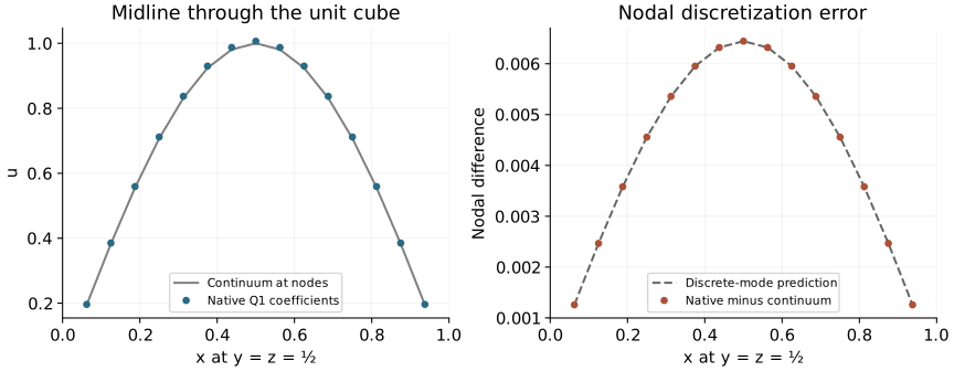
The figure reads native C++ coefficients. The checker visits every free node from every rank and compares it with \(\alpha_h s\). It separately measures the nodal difference from \(s\). Neither the plotted midline nor the scalar solver residual replaces that complete-field check.

For the Poisson case \(D=1,c=0\), the small supplied grids give

Free nodes per axis	\(h\)	\(|\alpha_h-1|\)
\(15\)	\(1/16\)	\(6.44\times10^{-3}\)
\(31\)	\(1/32\)	\(1.61\times10^{-3}\)

Halving the spacing reduces this nodal difference by about four, consistent with its \(O(h^2)\) expansion. This is a nodal error for the selected smooth mode; it is not an integrated error norm of the interpolated finite-element function or a convergence result for arbitrary geometries.

Run the weak problem and refine its grid

From the repository root, with a compatible installed CPU SDK:

openpfc run examples/finite-elements/q1-multigrid/model.cpp examples/finite-elements/q1-multigrid/input.json

The CLI prints its saved attempt directory. Inspect results/run.json and results/field_rank_*.csv below that directory. Add --ranks 2 --launcher=mpirun to the source-run command for the supported two-rank decomposition; invoke the CLI once outside the launcher.

The complete model and input need no private helper headers. Its CMake target is q1_multigrid.

Change n from 15 to 31 and compare the predicted nodal discretization error separately from the residual. Then set reaction to 1 and update both the forcing and discrete-eigenvalue prediction through the supplied parameters. Tightening the CG tolerance further should not remove the finite-element error relative to the continuum.

References

Brenner, Susanne C., and L. Ridgway Scott. 2008. The Mathematical Theory of Finite Element Methods. 3rd ed. Springer. https://doi.org/10.1007/978-0-387-75934-0.