A stencil has moments, units and a boundary contract

Finite differences / Give the weights a meaning

A stencil has moments, units and a boundary contract

Two implementations can agree perfectly and still apply the wrong normalization. Test what the weights mean.

Download runnable lesson (.zip)

Includes the model, inputs, required headers and a short run guide.

The centered first difference uses weights \(d=(-1,0,1)/(2h)\). Their sum is zero, so constants disappear; their first spatial moment is one, so the derivative of \(u=x\) is one.

The three-dimensional Sobel-x kernel combines a difference along x with smoothing in y and z. The raw integer coefficients \((-1,0,1)\otimes(1,2,1)\otimes(1,2,1)\) need a factor \(1/(32h)\): the difference contributes \(2h\), and each smoothing vector sums to four. The old example’s raw kernel was therefore 32, not 16, times its unit-spacing central-difference response on a transversely constant field.

Normalize each factor

Use the physical derivative weights and unit-sum smoothing weights:

const std::array derivative{-0.5 / h, 0.0, 0.5 / h};
const std::array smoothing{0.25, 0.5, 0.25};
double weights[3][3][3];
for (int k = 0; k < 3; ++k)
  for (int j = 0; j < 3; ++j)
    for (int i = 0; i < 3; ++i)
      weights[k][j][i] = derivative[i] * smoothing[j] * smoothing[k];

The dense box stores the same tensor product as the separable call. It is indexed [z][y][x]. The last direction is contiguous in the backing brick.

Apply three public kernels

const double central = stencil::apply_1d_along<0>(derivative.data(), 1,
                                                  u.data(), c, sx, sy, sz);
const double separable =
    stencil::apply_separable(derivative.data(), 1, smoothing.data(), 1,
                             smoothing.data(), 1, u.data(), c, sx, sy, sz);
const double dense =
    stencil::apply_dense(weights, u.data(), c, sx, sy, sz);

central differentiates only along x. separable differentiates along x and smooths in the two transverse directions. dense applies the same 27-point tensor weights directly. Equality of the last two checks their implementation parity; it does not by itself prove the intended derivative.

Each kernel takes a pointer, a center offset and explicit strides. A single offset lambda describes the sample brick; all three calls use that same layout.

Ask a polynomial for the truncation error

Choose

\[ \begin{gathered} u=x^3+xy^2+\tfrac12xz^2,\\ u_x=3x^2+y^2+\tfrac12z^2. \end{gathered} \]

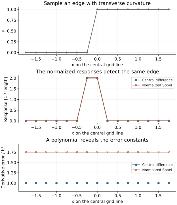
The central difference differentiates \(x^3\) as \(3x^2+h^2\). A normalized \((1,2,1)\) average maps \(y^2\) to \(y^2+h^2/2\). Applying those two identities in the tensor product gives

\[ \begin{gathered} D_xu=u_x+h^2,\\ S_xu=u_x+\tfrac74h^2. \end{gathered} \]

Both formulas are second order. The smoothing changes the error constant; it is not a universal improvement in derivative accuracy.

Figure 1: Native edge samples and the two normalized responses, followed by their polynomial errors divided by the squared spacing. Dense and separable Sobel responses agree; the independent polynomial argument predicts the error constants.

Decide where a stencil is defined

The output contains all \((N-2)^3\) interior nodes. The one-cell outer layer is excluded because a radius-one kernel would load outside the array. Excluding it is not a physical boundary condition.

For distributed data, the one-axis kernel needs its corresponding halo. The tensor stencil also reaches edge and corner neighbors: a face-only halo exchange is insufficient. Use a corner-filled policy such as host HaloConnectivity::Full before applying these multi-axis kernels. The separate-halo heat example has a face-neighbor Laplacian and a different support requirement.

Change the sampled field

openpfc run model.cpp input.json --launcher=none

The model and input need no companion header. The default is a step across x, multiplied by a smooth quadratic amplitude in y and z. Set profile to affine to calibrate the normalization, or polynomial to check the exact \(h^2\) error above. The bundled polynomial input selects that case directly.

spacing is physical distance between samples. This is a bounded sampled brick, with width \((N-1)h\) and both endpoint samples retained; it does not assume FFT periodicity. To refine the same physical interval, halve spacing and replace \(N\) by \(2N-1\).

Each attempt writes the complete interior to results/responses.csv. The checker invokes the actual binary for all three profiles and two polynomial resolutions. It checks every interior response against the affine and polynomial moment identities, including the spacing factor, sign, transverse curvature, unique grid coverage and invalid inputs. Run this demonstrator on a single CPU process.