Boundaries / Give a flux its direction and units
Count what leaves the boundary
A small diffusion problem. Two equivalent boundary inputs. One closed budget.
Download runnable lesson (.zip)
Includes the model, inputs, required headers and a short run guide.
Periodic Fourier grids identify opposite sides. Here the interval has two physical ends. Consider constant-coefficient diffusion on \(0\le x\le1\):
\[ u_t=D u_{xx},\qquad D>0. \]
The diffusive flux vector is \(-D u_x\). Its outward scalar component is different at the two ends because their normals point in opposite directions:
\[ J_L=D u_x(0,t),\qquad J_R=-D u_x(1,t). \]
Integrating the equation therefore gives
\[ \frac{d}{dt}\int_0^1u\,dx=-(J_L+J_R). \]
Positive outward flux removes inventory. Equal positive values at the two ends do not cancel.
Choose a solution you can differentiate
Let \(A\) be a constant and take
\[ u(x,t)=1+A x(1-x)-2DA t. \]
Its second derivative is \(-2A\) and its time derivative is \(-2DA\), so it solves the diffusion equation exactly. At both ends, the outward normal derivative is \(-A\), and the physical outward flux is \(DA\). Those quantities have different units and opposite signs when \(A>0\).
The model accepts either representation explicitly:
using pfc::field::fd::BoundaryQuantity;
const bool prescribe_flux = p.boundary == "flux";
const pfc::field::fd::FaceCondition face{
    prescribe_flux ? BoundaryQuantity::ConstitutiveFlux
                   : BoundaryQuantity::NormalDerivative,
    [=](double) {
      return prescribe_flux ? p.diffusivity * p.amplitude : -p.amplitude;
    }};
FaceCondition::flux converts an outward normal derivative \(q\) to \(-Dq\); it uses a constitutive flux directly. Supplying \(DA\) as a derivative would ask for a different boundary condition.
Let the operator own its boundary closure
DiffusionAxis supplies the nonperiodic finite-difference closure and a positive diagonal quadrature norm \(H\). Summation-by-parts operators retain a discrete integration-by-parts identity; Mattsson (2012) gives the variable- coefficient construction underlying this family.
For spacing \(h\), the first four norm weights are
\[ h\,(17,59,43,49)/48, \]
mirrored at the right end, with weight \(h\) in the interior. The operator requires at least 17 nodes so its boundary closures do not overlap. Our inventory is
\[ M_h=\sum_i H_{ii}u_i. \]
Using an unweighted sum, or replacing these weights with a trapezoidal rule, would measure a different discrete inventory. The operator reads state and material through global-axis callbacks. This one-dimensional example owns every node on one MPI rank; the axis itself performs no communication.
Advance the state and account for the accepted flux
for (int step = 0; step < steps; ++step) {
  const double time = step * dt;
  for (int i = 0; i < p.n; ++i) {
    const double rhs = axis.apply(
        i, [&](int j) { return u[j]; }, [&](int) { return p.diffusivity; }, time,
        &face, &face);
    next[i] = u[i] + dt * rhs;
  }
  ledger.begin();
  ledger.stage(face.flux(time, p.diffusivity), 1.0, dt);
  ledger.stage(face.flux(time, p.diffusivity), 1.0, dt);
  u.swap(next);
  ledger.accept();
  observe(step + 1);
}
Every right-hand-side evaluation reads the old state, and only then swaps in the new vector. FluxLedger::stage receives flux, face measure and time weight. Each endpoint of this one-dimensional interval has measure one. The two stages account for the two faces of a single Euler step, not two Runge–Kutta stages.
The ledger commits an accepted step’s outward integral. Its public reject operation discards a trial integral; an adaptive caller would also restore its trial state. This lesson uses fixed accepted steps and does not claim an adaptive rollback mechanism.
The model chooses \(\Delta t\le0.02h^2/D\) and adjusts it to reach the requested final time exactly. This is a conservative choice for this small explicit demo, not a general stability bound for other operators or integrators.
Check both the shape and the inventory
The norm integrates this quadratic exactly, giving
\[ \begin{aligned} M_h(0)&=1+A/6,\\ M_h(t)&=1+A/6-2DA t,\\ \mathcal J(t)&=2DA t. \end{aligned} \]
Consequently \(M_h(t)+\mathcal J(t)=M_h(0)\). The quadratic spatial derivative and its constant time tendency are reproduced up to floating point effects. This example tests boundary signs, closure and accounting; it is not an observed-order study for general smooth solutions.
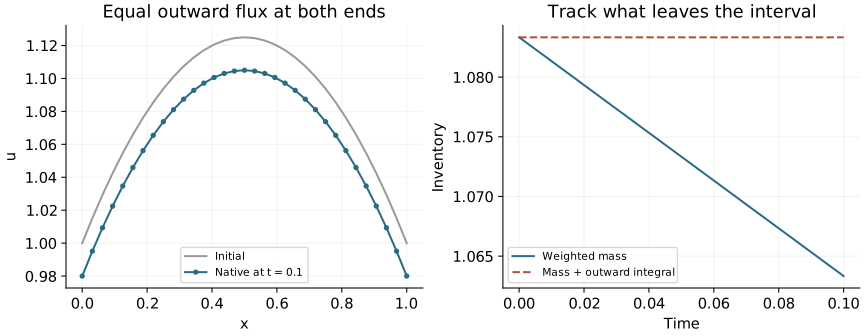
The figure reads native C++ CSV output. The checker compares every node with the analytic quadratic and every budget row with the closed-form inventory, including equivalent flux/derivative inputs and an inflow case. A correct scalar budget alone would not establish a correct field.
Run, change a sign and predict the result
From the repository root, with a compatible installed CPU SDK:
openpfc run examples/boundaries/outward-flux/model.cpp examples/boundaries/outward-flux/input.jsonThe CLI prints the saved attempt directory; its results/ contains the outputs. The supplied parameters are in input.json. To keep experiments separate, compile once and run from your own result directory:
mkdir -p results/outward-flux
openpfc compile examples/boundaries/outward-flux/model.cpp -o results/outward-flux/model
cp examples/boundaries/outward-flux/input.json results/outward-flux/input.json
cd results/outward-flux
./model input.json
The complete model needs no private helper header. It writes results/field.csv, results/budget.csv and results/run.json below the working directory. Its CMake target is outward_diffusion_flux.
Set boundary to derivative: the solution should stay the same because the input represents the same physical condition. Then use negative amplitude and predict the sign of both outward fluxes and the inventory change. Vary diffusivity, keeping its value positive, and distinguish the change in physical decay from the smaller explicit timestep.